This is a notebook I wrote while working on a project to classify WSF ferry alerts using scikit-learn. The output of each cell is rendered below the cell as it is in the notebook. See the project writeup here.
Uses Scikit-learn to train a Support Vector Machine (SVM) to classify WSF alerts.
Preprocess data
Load data and categories
%matplotlib inline
import pandas as pd


rawData = pd.read_csv('db-dump.csv')

# Drop predictions column
data = rawData.drop('prediction', axis=1)
data = data.dropna()

# drop rows with audit_count == 0
data = data[data.audit_count != 0]
data.head()
Matplotlib is building the font cache; this may take a moment.| bulletinid | alert | alert_category | audit_count | |
|---|---|---|---|---|
| 0 | 80227 | {\n "IVRText": null,\n "SortSeq": 2,\n "Ale... | high_priority_vessel | 2 |
| 1 | 80228 | {"IVRText": null, "SortSeq": 2, "AlertType": "... | high_priority_vessel | 2 |
| 2 | 80223 | {\n "IVRText": null,\n "SortSeq": 2,\n "Ale... | sailing_cancellation | 2 |
| 3 | 80333 | {"IVRText": null, "SortSeq": 3, "AlertType": "... | low_priority_alert | 2 |
| 4 | 80072 | {"IVRText": null, "SortSeq": 2, "AlertType": "... | high_priority_vessel | 2 |
Extract the categories from the Dataframe
categories = [
 'low_priority_alert',
 'normal_priority_alert',
 'high_priority_vessel',
 'high_priority_terminal',
 'sailing_cancellation'
 ]

categories
['low_priority_alert',
'normal_priority_alert',
'high_priority_vessel',
'high_priority_terminal',
'sailing_cancellation']Convert alert text to numerical features
import string
from nltk.tokenize import word_tokenize
from nltk.corpus import stopwords
from nltk.stem import PorterStemmer
from sklearn.feature_extraction.text import TfidfVectorizer


# strip and tokenize
data['alert'] = data['alert'].apply(lambda x: x.lower())
data['alert'] = data['alert'].apply(lambda x: x.translate(str.maketrans('', '', string.punctuation)))
data['alert'] = data['alert'].apply(lambda x: word_tokenize(x))

# Remove stop words and stem the words
stop_words = set(stopwords.words('english'))
data['alert'] = data['alert'].apply(lambda x: [word for word in x if word not in stop_words])

stemmer = PorterStemmer()
data['alert'] = data['alert'].apply(lambda x: [stemmer.stem(word) for word in x])

# Convert the preprocessed alert data to numerical vectors
vectorizer = TfidfVectorizer()
X = vectorizer.fit_transform(data['alert'].apply(lambda x: ' '.join(x)))
y = data['alert_category']
z = data['bulletinid']

data['alert'].head()
0    [ivrtext, null, sortseq, 2, alerttyp, alert, b...
1    [ivrtext, null, sortseq, 2, alerttyp, alert, b...
2    [ivrtext, null, sortseq, 2, alerttyp, alert, b...
3    [ivrtext, null, sortseq, 3, alerttyp, alert, b...
4    [ivrtext, null, sortseq, 2, alerttyp, alert, b...
Name: alert, dtype: object
Split data into training and test sets
from sklearn.model_selection import train_test_split


X_train, X_test, y_train_labels, y_test_labels, id_train, id_test = train_test_split(X, y, z, test_size=0.4, random_state=42)

print('Train:', len(X_train.toarray()), '\n Test:', len(X_test.toarray()))
# print the first row of the training data
print(X_train.shape)
Train: 1524
Test: 1017
(1524, 9157)Encode labels
from sklearn.preprocessing import LabelEncoder


le = LabelEncoder()
le.fit(categories)
y_train = le.transform(y_train_labels)
y_test = le.transform(y_test_labels)
le.classes_
array(['high_priority_terminal', 'high_priority_vessel',
       'low_priority_alert', 'normal_priority_alert',
       'sailing_cancellation'], dtype='<U22')
Train and score SVM
from sklearn.svm import SVC


clf = SVC(kernel="linear", probability=True)
clf.fit(X_train, y_train)
y_pred = clf.predict(X_test)
score = clf.score(X_test, y_test)
score0.9508357915437562Learning curve
from sklearn.model_selection import LearningCurveDisplay


LearningCurveDisplay.from_estimator(clf, X, y, cv=5)
<sklearn.model_selection._plot.LearningCurveDisplay at 0x30455a660>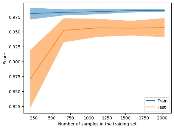
Cross Validation
from sklearn.model_selection import cross_val_score
scores = cross_val_score(clf, X, y, cv=5)

print("%0.2f accuracy with a standard deviation of %0.2f" % (scores.mean(), scores.std()))
0.96 accuracy with a standard deviation of 0.02Confusion matrix
from matplotlib import pyplot as plt
from sklearn.metrics import confusion_matrix
import seaborn as sns


cm = confusion_matrix(y_test, y_pred)
plt.figure(figsize=(5,3))
sns.heatmap(cm, annot=True, yticklabels=categories, xticklabels=categories, fmt='d')
plt.ylabel('Actual')
plt.xlabel('Predicted')
plt.title('Score: ' + str(round(score, 2)))
Text(0.5, 1.0, 'Score: 0.95')
Classification report
from sklearn.metrics import classification_report


print(classification_report(y_test, y_pred, target_names=categories))
precision recall f1-score support
low_priority_alert 1.00 1.00 1.00 150
normal_priority_alert 0.98 0.99 0.99 368
high_priority_vessel 0.95 0.85 0.89 110
high_priority_terminal 0.89 0.92 0.90 228
sailing_cancellation 0.92 0.94 0.93 161
accuracy 0.95 1017
macro avg 0.95 0.94 0.94 1017
weighted avg 0.95 0.95 0.95 1017-
The precision is the ratio
tp / (tp + fp)wheretpis the number of true positives andfpthe number of false positives. The precision is intuitively the ability of the classifier not to label a negative sample as positive. -
The recall is the ratio
tp / (tp + fn)wheretpis the number of true positives andfnthe number of false negatives. The recall is intuitively the ability of the classifier to find all the positive samples. -
The F-beta score can be interpreted as a weighted harmonic mean of the precision and recall, where an F-beta score reaches its best value at 1 and worst score at 0.
-
The support is the number of occurrences of each class in
y_true.
Principle Component Analysis
Reduce the dimensionality of the data and plot the results. This is mostly for fun (?)
from sklearn.decomposition import PCA


pca = PCA(n_components=2)
X_train_pca = pca.fit_transform(X_train.toarray())
plt.figure(figsize=(7, 5))
plt.title('PCA of the training data')
sns.scatterplot(x=X_train_pca[:, 0], y=X_train_pca[:, 1], hue=y_train_labels, palette=sns.color_palette('husl', len(categories)))
plt.show()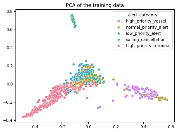
Analyze the misclassified alerts
Plot misclassified alerts with predictions and annotations
# plot the correlation between probability and actual category
y_pred_prob = clf.predict_proba(X_test)
y_pred_prob = pd.DataFrame(y_pred_prob)

# Predicted category is the highest probability of the 5 categories
y_pred_prob['predicted'] = le.classes_[y_pred_prob.idxmax(axis=1)]

y_pred_prob['actual'] = y_test_labels.tolist()
y_pred_prob['bulletinid'] = id_test.tolist()

# add the alert for a given bulletinid
y_pred_prob = y_pred_prob.merge(rawData[['bulletinid', 'alert']], on='bulletinid', how='left')

# filter for misclassified alerts
y_pred_prob = y_pred_prob[y_pred_prob['actual'] != y_pred_prob['predicted']]

# set column labels for categories
y_pred_prob.columns = [le.classes_.tolist() + ['predicted', 'actual', 'bulletinid', 'alert']]

# y_pred_prob.to_csv('misclassified.csv', index=False)
# len(y_pred_prob)
# show just bulletinid and alert
y_pred_prob.to_csv('misclassified.csv', index=False)
Export model for use in the API
from joblib import dump
from sklearn.pipeline import Pipeline


# Build a pipeline to preprocess input data and predict the category
tfidf_svm = Pipeline([('tfidf', vectorizer), ('svm', clf)])
dump(tfidf_svm, 'out/model.joblib')
['out/model.joblib']